graph LR
    CurrenyChoice[Project] --- Data[Data]
    CurrenyChoice --- Code[Code]
    CurrenyChoice --- Figures[Figures]
    CurrenyChoice --- Tables[Tables]
    CurrenyChoice --- Texts[Texts]
    CurrenyChoice --- References[References]
    CurrenyChoice --- Tasks[Tasks]
    Data --- In[In]
    Data --- Out[Out]
    Code --- R[R]
    Code --- Julia[Julia]
    R --- ROld[Old]
    Texts --- Notes[Notes]
    Texts --- Slides[Slides]
    Texts --- Paper[Paper]
    Notes --- Summary[Summary]
    Notes --- Readme[README]
    References --- Bib[Bibs]
    Summary --- SOld[Old]
RA Instructions
General rules
- Avoid space or “()” in output file names (especially .tex, .pdf files), use “_” instead (to avoid potential compilation problems in LaTeX).
- Be careful about the file name to avoid overwriting the existing files. If necessary, create subfolders for different tasks.
- Always ask questions if you are not sure.
Folder Structure
- Data/ folder
- In/ folder: raw data
- Direct download from open sources
- No modification except for renaming the file name
- E.g., can’t edit Excel files, can’t manually convert Excel to CSV, etc
- Out/ folder: processed data
- Direct output from code files
- Manually modified data (e.g., manually adjust the common languages, colonial relationship, etc). Not recommended, but sometimes necessary.
- In/ folder: raw data
- Code/ folder
- R/ folder: R scripts (.R)
- Mainly used for data processing, running regressions, generating tables (.tex) and figures (.pdf)
- Old/ folder: old R scripts that are not used anymore (but still keep them for reference)
- Julia/ folder: Julia scripts (.jl) and Juptyer notebooks
- Mainly used for carrying out counterfactual analysis and simulations
- R/ folder: R scripts (.R)
- Tables folder
- Regression tables and summary statistics tables (.tex) that can be directly inserted into the LaTeX files. Rarely have other file types.
- In the future, create subfolders when outputting tables for different tasks
- Figures folder
- Figures (.pdf) that can be directly inserted into the LaTeX files. Rarely have other file types.
- In the future, create subfolders when outputting figures for different tasks
- References/ folder
- Relevant literature.
- Rules of the filenames (suggested by Keith)
- Two authors: Author1Author2YEARJournal abbrev keywords.pdf, e.g., HeadMayer2019AER_cars.pdf
- Three or more authors: Author1 etalYEARJournal abbrev keywords.pdf, e.g., Amiti_etal2020NBER_DominantCurrencies.pdf
- Sometimes initials are better known, e.g., ACR2012AER.pdf for the Arkolakis, Costinot and Rodriguez-Clare paper on “same old gains” in AER.
- Bibs/ folder: bib files, which are used to generate the bibliography in LaTeX files
- literature_review_all.bib: latest version of the bib file we currently use.
- Rules of the tags: As with the file names but skip the keywords, e.g., HeadMayer2019AER, Amiti_etal2020NBER, ACR2012AER
- Text/ folder
- Notes/ folder: general notes
- LaTeX(.tex), Word (.docx) and text (.txt) files
- Summary/ folder: summary of the current work. Updated when needed.
- Old/ folder: old summary files, including both old versions of .tex and .pdf files (rename the file name to indicate the date)
- Slides/ folder: slides for presentations
- Paper/ folder: draft of the paper
- Notes/ folder: general notes
- Tasks/ folder
- Task allocations and descriptions
Instruction for README file
Start a new LaTeX file and note down the following information in Notes/README:
- Construction of the data sets (refer to Section 4 in the old readme file).
- code, input dataset, output dataset, and brief description (data sources, reference, data cleaning steps, etc).
- Figures and table generation (refer to Section 5 in the old readme file).
R tutorial (in progress)
Output figures
Simulation code
library(data.table)
library(HeadR)
library(basicPlotteR)
# Simulating data
set.seed(123) # For reproducibility
x <- rnorm(100) # 100 random numbers from a normal distribution
y <- 2*x + rnorm(100) # Creating a linear relationship with some added noise
z <- sample(letters[1:4], 100, replace = TRUE) # Creating a categorical variable
DT <- data.table(x, y, z) # Creating a data.tablepdf("Figures/R_example1.pdf", 6,8) # set the output file name and size
par(mar=c(4,4,1,1)+0.1) # set the margin
# Creating a scatter plot using HeadR::scatter function, or use base R plot function
scatter(x, y, xlab = "X", ylab = "Y", pch = 19, col = "blue")
addTextLabels(DT$x, DT$y , DT$z , cex.label = 0.7, col.label = "black")
ols <- lm(y ~ x, data = DT) # OLS regression
lines(DT$x, predict(ols), col = "red") # OLS line
lbl1 <- paste("slope = ", round(ols$coefficients[2], 2), " (p = 0.06)")
lbl2<- paste("R^2 = ", round(summary(ols)$r.squared, 3), ", RMSE = ", round(sigma(ols), 2),sep = "")
# add the coefficient and R^2 of the regression line as legend
legend("topleft", c(lbl1, lbl2), lty = c("solid", NA), col = c("red", NA), lwd = 2)
dev.off()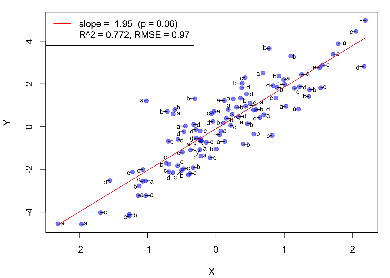
Output tables
Simulation code
library(data.table)
library(HeadR)
# Simulating data
set.seed(123) # For reproducibilit
DT <- CJ(i=1:10,t=1:20) # cross-join function CJ() makes a panel of 100 individuals observe 20 periods each
DT[, income := rlnorm(10*20)] # log-normal income data
DT[ , income_life := mean(income), by=i] # average income over the life cycle, assign to each individual
DTi <- DT[ , .(income_life = mean(income)), by=i]
# alternative: DTi <- unique(DT[, .(i, income_life)]
# use texout to generate a column for LaTeX output
DTi[, output := texout(list(i, income_life), digits = 3)] # default digits = 2
DTi$output [1] "1 & 1.766 \\\\" "2 & 1.275 \\\\" "3 & 1.765 \\\\" "4 & 1.404 \\\\"
[5] "5 & 2.053 \\\\" "6 & 0.873 \\\\" "7 & 1.672 \\\\" "8 & 1.411 \\\\"
[9] "9 & 2.667 \\\\" "10 & 1.377 \\\\"# Output to a tex file using writeLines()
writeLines(DTi$output, "Tables/R_example2.tex")Output regression tables
Simulation code
library(data.table)
library(fixest)
library(MASS)
gamma_x <- 0.333
gamma_N <- 0.667
nobs <- 1e5
rho <- -0.5
set.seed(5772) #eulers gamma constant
ld <- exp(rnorm(nobs,mean=1,sd=0.5))
# Define the mean and the covariance matrix
mu <- c(0, 0)  # means
Sigma <- matrix(c(0.25^2, rho*0.25*0.25, rho*0.25*0.25, 0.25^2), ncol=2)  # covariance matrix
# Generate bivariate log normal variates
bilnorm <- exp(mvrnorm(nobs, mu, Sigma))
u_x <- bilnorm[, 1]
u_N <- bilnorm[, 2]
x <- exp(gamma_x*ld)*u_x
N <- exp(gamma_N*ld)*u_N
X <- x*N
DT <- data.table(x=x, N=N, X=X, ld=ld)
# run regressions with fixest package
# here we use fepois() to run PPML regressions
# OLS will use feols()
res_N <- fepois(N ~ ld, data=DT)
res_x <- fepois(x ~ ld, data=DT)
res_X <- fepois(X ~ ld, data=DT)
# output regression tables to a tex file using etable()
# use a, b, c to indicate significance levels instead of stars
etable(res_N, res_x, res_X, file = "Tables/R_example3.tex",
signif.code = "letters", fitstat=~n+sq.cor+pr2, digits.stats = 3, digits = 3, replace =TRUE,
dict = c(`ld` = "Log distance", `x` = "Average trade flows", `N` = "Number of firms", `X` = "Total trade flows"))
# print the regression tables in the console
etable(res_N, res_x, res_X,
signif.code = "letters", fitstat=~n+sq.cor+pr2,digits.stats = 3, digits = 3, replace =TRUE,
dict = c(`ld` = "Log distance", `x` = "Average trade flows", `N` = "Number of firms", `X` = "Total trade flows")) res_N res_x res_X
Dependent Var.: Number of firms Average trade flows Total trade flows
Constant -0.021a (0.001) 0.041a (0.003) -0.076a (0.0002)
Log distance 0.673a (7.18e-5) 0.331a (0.0005) 1.01a (1.16e-5)
_______________ ________________ ___________________ _________________
S.E. type IID IID IID
Observations 100,000 100,000 100,000
Squared Cor. 0.989 0.938 0.996
Pseudo R2 0.990 0.449 0.999
---
Signif. codes: 0 'a' 0.01 'b' 0.05 'c' 0.1 ' ' 1R learning sources
- Keith’s blogs: 1, 2
- Keith’s R Google doc
- Introduction to fixest
- A good course
LaTeX tutorial (in progress)
A template for LaTeX files is provided in the Text/Notes/ folder. Some useful commands are listed below.
% input tex table
\input{Tables/R_example3.tex}